动态规划

Dynamic programming

From Wikipedia, the free encyclopedia 

In mathematics and computer science, dynamic programming is a method of solving complex problems by breaking them down into simpler steps. It is applicable to problems that exhibit the properties of overlapping subproblems and optimal substructure (described below). When applicable, the method takes much less time than naive methods.

Bottom-up dynamic programming simply means storing the results of certain calculations, which are then re-used later because the same calculation is a sub-problem in a larger calculation. Bottom-up dynamic programming involves formulating a complex calculation as a recursive series of simpler calculations.

Contents

• 1 History
• 2 Overview
  • 2.1 Dynamic programming in mathematical optimization
  • 2.2 Dynamic programming in computer programming
• 3 Example: mathematical optimization
  • 3.1 Optimal consumption and saving
• 4 Examples: Computer algorithms
  • 4.1 Fibonacci sequence
  • 4.2 A type of balanced 0-1 matrix
  • 4.3 Checkerboard
  • 4.4 Sequence alignment
• 5 Algorithms that use dynamic programming
• 6 See also
• 7 References
• 8 Further reading
• 9 External links

History

The term was originally used in the 1940s by Richard Bellman to describe the process of solving problems where one needs to find the best decisions one after another. By 1953, he had refined this to the modern meaning, which refers specifically to nesting smaller decision problems inside larger decisions,and the field was thereafter recognized by the IEEE as a systems analysis and engineering topic. Bellman's contribution is remembered in the name of the Bellman equation, a central result of dynamic programming which restates an optimization problem in recursive form.

Originally the word "programming" in "dynamic programming" had no connection to computer programming, and instead came from the term "mathematical programming"^[2] - a synonym for optimization. However, nowadays many optimization problems are best solved by writing a computer program that implements a dynamic programming algorithm, rather than carrying out hundreds of tedious calculations by hand. Some of the examples given below are illustrated using computer programs.

Overview

Figure 1. Finding the shortest path in a graph using optimal substructure; a straight line indicates a single edge; a wavy line indicates a shortest path between the two vertices it connects (other nodes on these paths are not shown); the bold line is the overall shortest path from start to goal.

Dynamic programming is both a mathematical optimization method, and a computer programming method. In both contexts, it refers to simplifying a complicated problem by breaking it down into simpler subproblems in a recursive manner. While some decision problems cannot be taken apart this way, decisions that span several points in time do often break apart recursively; Bellman called this the "Principle of Optimality". Likewise, in computer science, a problem which can be broken down recursively is said to have optimal substructure.

If subproblems can be nested recursively inside larger problems, so that dynamic programming methods are applicable, then there is a relation between the value of the larger problem and the values of the subproblems.^[3] In the optimization literature this relationship is called the Bellman equation.

Dynamic programming in mathematical optimization

In terms of mathematical optimization, dynamic programming usually refers to a simplification of a decision by breaking it down into a sequence of decision steps over time. This is done by defining a sequence of value functions V₁ , V₂ , ... V_n , with an argument y representing the state of the system at times i from 1 to n. The definition of V_n(y) is the value obtained in state y at the last time n. The values V_i at earlier times i=n-1,n-2,...,2,1 can be found by working backwards, using a recursive relationship called the Bellman equation. For i=2,...n, V_{i -1} at any state y is calculated from V_i by maximizing a simple function (usually the sum) of the gain from decision i-1 and the function V_i at the new state of the system if this decision is made. Since V_i has already been calculated, for the needed states, the above operation yields V_{i -1} for all the needed states. Finally, V₁ at the initial state of the system is the value of the optimal solution. The optimal values of the decision variables can be recovered, one by one, by tracking back the calculations already performed.

Dynamic programming in computer programming

As a computer programming method, dynamic programming is mainly used to tackle problems that are solvable in polynomial time.There are two key attributes that a problem must have in order for dynamic programming to be applicable: optimal substructure and overlapping subproblems.

Optimal substructure means that the solution to a given optimization problem can be obtained by the combination of optimal solutions to its subproblems. Consequently, the first step towards devising a dynamic programming solution is to check whether the problem exhibits such optimal substructure. Such optimal substructures are usually described by means of recursion. For example, given a graph G=(V,E), the shortest path p from a vertex u to a vertex v exhibits optimal substructure: take any intermediate vertex w on this shortest path p. If p is truly the shortest path, then the path p₁ from u to w and p₂ from w to v are indeed the shortest paths between the corresponding vertices (by the simple cut-and-paste argument described in CLRS). Hence, one can easily formulate the solution for finding shortest paths in a recursive manner, which is what the Bellman-Ford algorithm does.

Overlapping subproblems means that the space of subproblems must be small, that is, any recursive algorithm solving the problem should solve the same subproblems over and over, rather than generating new subproblems. For example, consider the recursive formulation for generating the Fibonacci series: F_i = F_i-1 + F_i-2, with base case F₁=F₂=1. Then F₄₃ = F₄₂ + F₄₁, and F₄₂ = F₄₁ + F₄₀. Now F₄₁ is being solved in the recursive subtrees of both F₄₃ as well as F₄₂. Even though the total number of subproblems is actually small (only 43 of them), we end up solving the same problems over and over if we adopt a naive recursive solution such as this. Dynamic programming takes account of this fact and solves each subproblem only once.

Figure 2. The subproblem graph for the Fibonacci sequence. The fact that it is not a tree indicates overlapping subproblems.

This can be achieved in either of two ways:

• Top-down approach: This is the direct fall-out of the recursive formulation of any problem. If the solution to any problem can be formulated recursively using the solution to its subproblems, and if its subproblems are overlapping, then one can easily memoize or store the solutions to the subproblems in a table. Whenever we attempt to solve a new subproblem, we first check the table to see if it is already solved. If a solution has been recorded, we can use it directly, otherwise we solve the subproblem and add its solution to the table.

• Bottom-up approach: This is the more interesting case. Once we formulate the solution to a problem recursively as in terms of its subproblems, we can try reformulating the problem in a bottom-up fashion: try solving the subproblems first and use their solutions to build-on and arrive at solutions to bigger subproblems. This is also usually done in a tabular form by iteratively generating solutions to bigger and bigger subproblems by using the solutions to small subproblems. For example, if we already know the values of F₄₁ and F₄₀, we can directly calculate the value of F₄₂.

Some programming languages can automatically memoize the result of a function call with a particular set of arguments, in order to speed up call-by-name evaluation (this mechanism is referred to as call-by-need). Some languages make it possible portably (e.g. Scheme, Common Lisp or Perl), some need special extensions (e.g. C++, see ^[4]). Some languages have automatic memoize built in. In any case, this is only possible for a referentially transparent function.

Example: mathematical optimization

Optimal consumption and saving

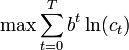
A mathematical optimization problem that is often used in teaching dynamic programming to economists (because it can be solved by hand: see Stokey et al., 1989, Chap. 1) concerns a consumer who lives over the periods t = 0,1,2,...,T and must decide how much to consume and how much to save in each period.

Let c_t be consumption in period t, and assume consumption yields utility u(c_t) = ln(c_t) as long as the consumer lives. Assume the consumer is impatient, so that he discounts future utility by a factor b each period, where 0 < b < 1. Let k_t be capital in period t. Assume initial capital is a given amount k₀ > 0, and suppose that this period's capital and consumption determine next period's capital as 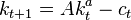, where A is a positive constant and 0 < a < 1. Assume capital cannot be negative. Then the consumer's decision problem can be written as follows:

subject to for all t = 0,1,2,...,T

Written this way, the problem looks complicated, because it involves solving for all the choice variables c₀,c₁,c₂,...,c_T and k₁,k₂,k₃,...,k_{T + 1} simultaneously. (Note that k₀ is not a choice variable—the consumer's initial capital is taken as given.)

The dynamic programming approach to solving this problem involves breaking it apart into a sequence of smaller decisions. To do so, we define a sequence of value functions V_t(k), for t = 0,1,2,...,T,T + 1 which represent the value of having any amount of capital k at each time t. Note that V_{T + 1}(k) = 0, that is, there is (by assumption) no utility from having capital after death.

The value of any quantity of capital at any previous time can be calculated by backward induction using the Bellman equation. In this problem, for each t = 0,1,2,...,T, the Bellman equation is

subject to

This problem is much simpler than the one we wrote down before, because it involves only two decision variables, c_t and k_{t + 1}. Intuitively, instead of choosing his whole lifetime plan at birth, the consumer can take things one step at a time. At time t, his current capital k_t is given, and he only needs to choose current consumption c_t and saving k_{t + 1}.

To actually solve this problem, we work backwards. For simplicity, the current level of capital is denoted as k. V_{T + 1}(k) is already known, so using the Bellman equation once we can calculate V_T(k), and so on until we get to V₀(k), which is the value of the initial decision problem for the whole lifetime. In other words, once we know V_{T − j + 1}(k), we can calculate V_{T − j}(k), which is the maximum of ln(c_{T − j}) + bV_{T − j + 1}(Ak^a − c_{T − j}), where c_{T − j} is the variable and . It can be shown that the value function at time t = T − j is

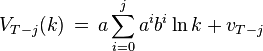
where each v_{T − j} is a constant, and the optimal amount to consume at time t = T − j is

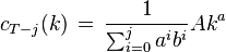
which can be simplified to

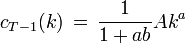, and , and 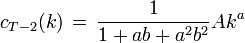, etcetera.

We see that it is optimal to consume a larger fraction of current wealth as one gets older, finally consuming all current wealth in period T, the last period of life.

[edit] Examples: Computer algorithms

[edit] Fibonacci sequence

Here is a naive implementation of a function finding the nth member of the Fibonacci sequence, based directly on the mathematical definition:

   function fib(n)
       if n = 0 return 0
       if n = 1 return 1
       return fib(n − 1) + fib(n − 2)

Notice that if we call, say, fib(5), we produce a call tree that calls the function on the same value many different times:

1. fib(5)
2. fib(4) + fib(3)
3. (fib(3) + fib(2)) + (fib(2) + fib(1))
4. ((fib(2) + fib(1)) + (fib(1) + fib(0))) + ((fib(1) + fib(0)) + fib(1))
5. (((fib(1) + fib(0)) + fib(1)) + (fib(1) + fib(0))) + ((fib(1) + fib(0)) + fib(1))

In particular, fib(2) was calculated three times from scratch. In larger examples, many more values of fib, or subproblems, are recalculated, leading to an exponential time algorithm.

Now, suppose we have a simple map object, m, which maps each value of fib that has already been calculated to its result, and we modify our function to use it and update it. The resulting function requires only O(n) time instead of exponential time:

   var m := map(0 → 0, 1 → 1)
   function fib(n)
       if map m does not contain key n
           m[n] := fib(n − 1) + fib(n − 2)
       return m[n]

This technique of saving values that have already been calculated is called memoization; this is the top-down approach, since we first break the problem into subproblems and then calculate and store values.

In the bottom-up approach we calculate the smaller values of fib first, then build larger values from them. This method also uses O(n) time since it contains a loop that repeats n − 1 times, however it only takes constant (O(1)) space, in contrast to the top-down approach which requires O(n) space to store the map.

   function fib(n)
       var previousFib := 0, currentFib := 1
       if n = 0 
           return 0
       else if n = 1 
           return 1
       repeat n − 1 times
           var newFib := previousFib + currentFib
           previousFib := currentFib
           currentFib  := newFib
       return currentFib

In both these examples, we only calculate fib(2) one time, and then use it to calculate both fib(4) and fib(3), instead of computing it every time either of them is evaluated.

[edit] A type of balanced 0-1 matrix

Consider the problem of assigning values, either zero or one, to the positions of an n x n matrix, n even, so that each row and each column contains exactly n / 2 zeros and n / 2 ones. For example, when n = 4, three possible solutions are:

+ - - - - +             + - - - - +                + - - - - +
| 0 1 0 1 |             | 0 0 1 1 |                | 1 1 0 0 |
| 1 0 1 0 |     and     | 0 0 1 1 |       and      | 0 0 1 1 |
| 0 1 0 1 |             | 1 1 0 0 |                | 1 1 0 0 |
| 1 0 1 0 |             | 1 1 0 0 |                | 0 0 1 1 |
+ - - - - +             + - - - - +                + - - - - +

We ask how many different assignments there are for a given n. There are at least three possible approaches: brute force, backtracking, and dynamic programming. Brute force consists of checking all assignments of zeros and ones and counting those that have balanced rows and columns (n / 2 zeros and n / 2 ones). As there are possible assignments, this strategy is not practical except maybe up to n = 6. Backtracking for this problem consists of choosing some order of the matrix elements and recursively placing ones or zeros, while checking that in every row and column the number of elements that have not been assigned plus the number of ones or zeros are both at least n / 2. While more sophisticated than brute force, this approach will visit every solution once, making it impractical for n larger than six, since the number of solutions is already 116963796250 for n = 8, as we shall see. Dynamic programming makes it possible to count the number of solutions without visiting them all.

We consider boards, where whose k rows contain n / 2 zeros and n / 2 ones. The function f to which memoization is applied maps vectors of n pairs of integers to the number of admissible boards (solutions). There is one pair for each column and its two components indicate respectively the number of ones and zeros that have yet to be placed in that column. We seek the value of (n arguments or one vector of n elements). The process of subproblem creation involves iterating over every one of possible assignments for the top row of the board, and going through every column, subtracting one from the appropriate element of the pair for that column, depending on whether the assignment for the top row contained a zero or a one at that position. If any one of the results is negative, then the assignment is invalid and does not contribute to the set of solutions (recursion stops). Otherwise, we have an assignment for the top row of the board and recursively compute the number of solutions to the remaining board, adding the numbers of solutions for every admissible assignment of the top row and returning the sum, which is being memoized. The base case is the trivial subproblem, which occurs for a board. The number of solutions for this board is either zero or one, depending on whether the vector is a permutation of n / 2 (0,1) and n / 2 (1,0) pairs or not.

For example, in the two boards shown above the sequences of vectors would be

((2, 2) (2, 2) (2, 2) (2, 2))       ((2, 2) (2, 2) (2, 2) (2, 2))     k = 4
  0      1      0      1              0      0      1      1

((1, 2) (2, 1) (1, 2) (2, 1))       ((1, 2) (1, 2) (2, 1) (2, 1))     k = 3
  1      0      1      0              0      0      1      1

((1, 1) (1, 1) (1, 1) (1, 1))       ((0, 2) (0, 2) (2, 0) (2, 0))     k = 2
  0      1      0      1              1      1      0      0

((0, 1) (1, 0) (0, 1) (1, 0))       ((0, 1) (0, 1) (1, 0) (1, 0))     k = 1
  1      0      1      0              1      1      0      0

((0, 0) (0, 0) (0, 0) (0, 0))       ((0, 0) (0, 0), (0, 0) (0, 0))

The number of solutions (sequence A058527 in OEIS) is

Links to the Perl source of the backtracking approach, as well as a MAPLE and a C implementation of the dynamic programming approach may be found among the external links.

[edit] Checkerboard

Consider a checkerboard with n × n squares and a cost-function c(i, j) which returns a cost associated with square i,j (i being the row, j being the column). For instance (on a 5 × 5 checkerboard),

5 4 3 2 1   1 2 3 4 5

6	7	4	7	8
7	6	1	1	4
3	5	7	8	2
-	6	7	0	-
-	-	5*	-	-

Thus c(1, 3) = 5

Let us say you had a checker that could start at any square on the first rank (i.e., row) and you wanted to know the shortest path (sum of the costs of the visited squares are at a minimum) to get to the last rank, assuming the checker could move only diagonally left forward, diagonally right forward, or straight forward. That is, a checker on (1,3) can move to (2,2), (2,3) or (2,4).

5 4 3 2 1   1 2 3 4 5

	x	x	x
		o

This problem exhibits optimal substructure. That is, the solution to the entire problem relies on solutions to subproblems. Let us define a function q(i, j) as

q(i, j) = the minimum cost to reach square (i, j)

If we can find the values of this function for all the squares at rank n, we pick the minimum and follow that path backwards to get the shortest path.

Note that q(i, j) is equal to the minimum cost to get to any of the three squares below it (since those are the only squares that can reach it) plus c(i, j). For instance:

5 4 3 2 1   1 2 3 4 5

		A
	B	C	D

Now, let us define q(i, j) in somewhat more general terms:

The first line of this equation is there to make the recursive property simpler (when dealing with the edges, so we need only one recursion). The second line says what happens in the last rank, to provide a base case. The third line, the recursion, is the important part. It is similar to the A,B,C,D example. From this definition we can make a straightforward recursive code for q(i, j). In the following pseudocode, n is the size of the board, c(i, j) is the cost-function, and min() returns the minimum of a number of values:

function minCost(i, j)
    if j < 1 or j > n
        return infinity
    else if i = 5
        return c(i, j)
    else    
        return min( minCost(i+1, j-1), minCost(i+1, j), minCost(i+1, j+1) ) + c(i, j)

It should be noted that this function only computes the path-cost, not the actual path. We will get to the path soon. This, like the Fibonacci-numbers example, is horribly slow since it spends mountains of time recomputing the same shortest paths over and over. However, we can compute it much faster in a bottom-up fashion if we store path-costs in a two-dimensional array q[i, j] rather than using a function. This avoids recomputation; before computing the cost of a path, we check the array q[i, j] to see if the path cost is already there.

We also need to know what the actual shortest path is. To do this, we use another array p[i, j], a predecessor array. This array implicitly stores the path to any square s by storing the previous node on the shortest path to s, i.e. the predecessor. To reconstruct the path, we lookup the predecessor of s, then the predecessor of that square, then the predecessor of that square, and so on, until we reach the starting square. Consider the following code:

 function computeShortestPathArrays()
     for x from 1 to n
         q[1, x] := c(1, x)
     for y from 1 to n
         q[y, 0]     := infinity
         q[y, n + 1] := infinity
     for y from 2 to n
         for x from 1 to n
             m := min(q[y-1, x-1], q[y-1, x], q[y-1, x+1])
             q[y, x] := m + c(y, x) 
             if m = q[y-1, x-1]
                 p[y, x] := -1
             else if m = q[y-1, x]
                 p[y, x] :=  0
             else
                 p[y, x] :=  1

Now the rest is a simple matter of finding the minimum and printing it.

 function computeShortestPath()
     computeShortestPathArrays()
     minIndex := 1
     min := q[n, 1] 
     for i from 2 to n 
         if q[n, i] < min
             minIndex := i
             min := q[n, i]
     printPath(n, minIndex)

 function printPath(y, x)
     print(x)
     print("<-")
     if y = 2
         print(x + p[y, x])
     else
         printPath(y-1, x + p[y, x])

[edit] Sequence alignment

In genetics, sequence alignment is an important application where dynamic programming is essential ^[5]. Typically, the problem consists of transforming one sequence into another using edit operations that replace, insert, or remove an element. Each operation has an associated cost, and the goal is to find the sequence of edits with the lowest total cost.

The problem can be stated naturally as a recursion, a sequence A is optimally edited into a sequence B by either:

1. inserting the first character of B, and performing an optimal alignment of A and the tail of B
2. deleting the first character of A, and performing the optimal alignment of the tail of A and B
3. replacing the first character of A with the first character of B, and performing optimal alignments of the tails of A and B.

The partial alignments can be tabulated in a matrix, where cell (i,j) contains the cost of the optimal alignment of A[1..i] to B[1..j]. The cost in cell (i,j) can be calculated by adding the cost of the relevant operations to the cost of its neighboring cells, and selecting the optimum.

Different variants exist, see Smith-Waterman and Needleman-Wunsch.

[edit] Algorithms that use dynamic programming

• Backward induction as a solution method for finite-horizon discrete-time dynamic optimization problems
• Method of undetermined coefficients can be used to solve the Bellman equation in infinite-horizon, discrete-time, discounted, time-invariant dynamic optimization problems
• Many string algorithms including longest common subsequence, longest increasing subsequence, longest common substring, Levenshtein distance (edit distance).
• Many algorithmic problems on graphs can be solved efficiently for graphs of bounded treewidth or bounded clique-width by using dynamic programming on a tree decomposition of the graph.
• The Cocke-Younger-Kasami (CYK) algorithm which determines whether and how a given string can be generated by a given context-free grammar
• The use of transposition tables and refutation tables in computer chess
• The Viterbi algorithm (used for hidden Markov models)
• The Earley algorithm (a type of chart parser)
• The Needleman-Wunsch and other algorithms used in bioinformatics, including sequence alignment, structural alignment, RNA structure prediction.
• Floyd's All-Pairs shortest path algorithm
• Optimizing the order for chain matrix multiplication
• Pseudopolynomial time algorithms for the Subset Sum and Knapsack and Partition problem Problems
• The dynamic time warping algorithm for computing the global distance between two time series
• The Selinger (a.k.a. System R) algorithm for relational database query optimization
• De Boor algorithm for evaluating B-spline curves
• Duckworth-Lewis method for resolving the problem when games of cricket are interrupted
• The Value Iteration method for solving Markov decision processes
• Some graphic image edge following selection methods such as the "magnet" selection tool in Photoshop
• Some methods for solving interval scheduling problems
• Some methods for solving word wrap problems
• Some methods for solving the travelling salesman problem
• Recursive least squares method
• Beat tracking in Music Information Retrieval.
• Adaptive Critic training strategy for artificial neural networks
• Stereo algorithms for solving the Correspondence problem used in stereo vision.
• Seam carving (content aware image resizing)
• The Bellman-Ford algorithm for finding the shortest distance in a graph.
• Some approximate solution methods for the linear search problem.